Personalised XIRR and investing - part 2 (or how I learned to love pandas.merge_asof)
Recap from Part One
Part one of this two-part series motivated why you (as an investor) should be interested in XIRR (eXtended Internal Rate of Return) for all your investment portfolios. XIRR elegantly handles irregular cash flows in / out and provides an easy to understand, accurate reflection of investing performance - both at the individual stock and portfolio level. XIRR consider cash C invested for time T, when most other metrics just consider cash C which is much less useful.
In Part One, we built a proof of concept system that collects and formats investing transactions (buys, sells, dividends) so that the XIRR could be calculated. Just this functionality by itself has substantial value - as noted then, most investing platforms in the UK do not calculate or provide XIRR.
But Part One was ultimately just a stepping stone to Part Two - this article. Now we ask the hard question: could I have done better? Can I compare my individual decisions over time to simply investing in a passive tracker for the FTSE 100, S&P 500 or an All-World Tracker?
The reference data
Let’s focus on a “my portfolio” <> FTSE 100 comparison - the main index for the UK with about 70% of revenue derived from outside the UK. Large caps in the index include AstraZeneca, Rolls Royce, Shell, BP, the miners etc. The FTSE 100 is not exciting like the NASDAQ but it is respectable and a major benchmark for UK investors. It is usually worth about 4-5% of the total world equity (the USA is worth about 70% currently).
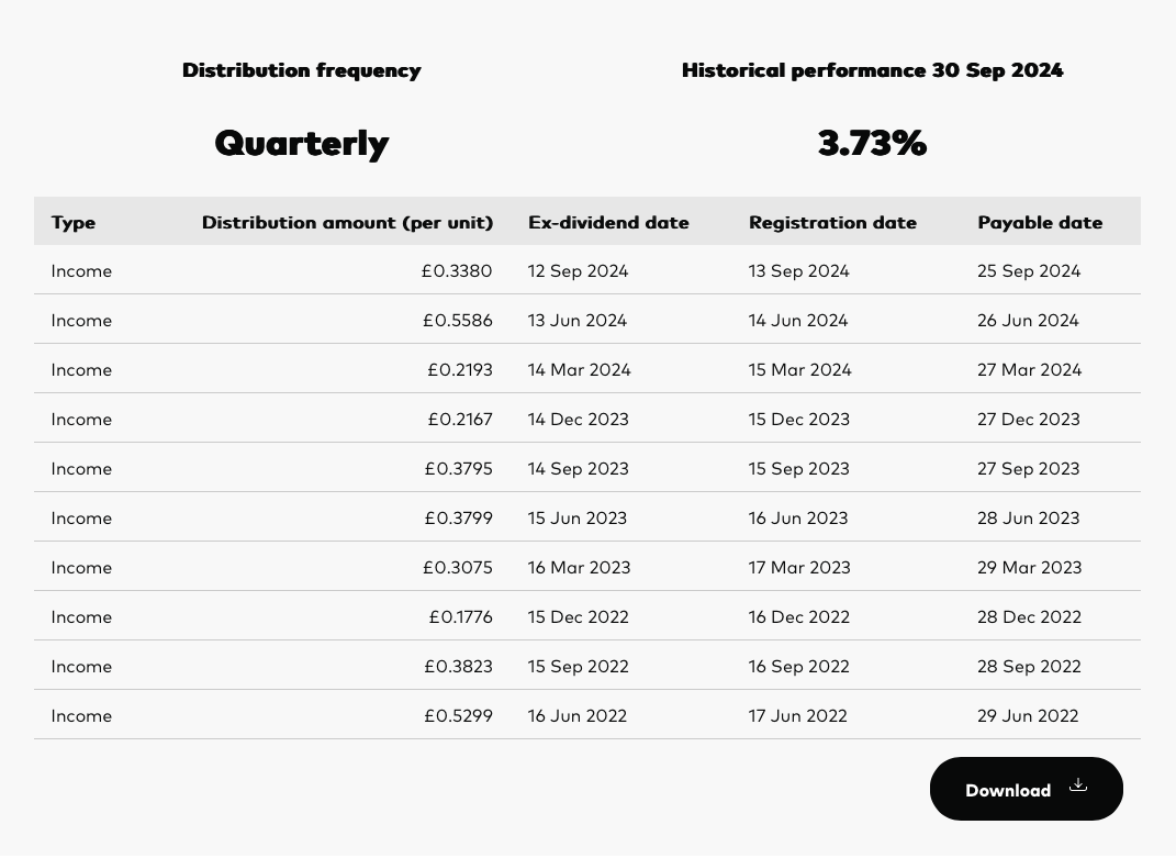
Vanguard is the 800-pound gorilla of index and ETF funds in the US and have established a significant footprint in the UK. Not only does Vanguard have an ETF which tracks the FTSE 100 - VUKE but they also release nightly drops of daily prices and quarterly distributions for this ETF in XLSX format.
This data is crucial for this post - when formatted correctly, it will form “DataFrame B” to act as the comparison to “DataFrame A” that we constructed in Part One.
Lastly, VUKE is also competitive from a charges standpoint - a real source of returns erosion for actively-managed funds. the Ongoing Charge or OCF for VUKE is 0.09%.
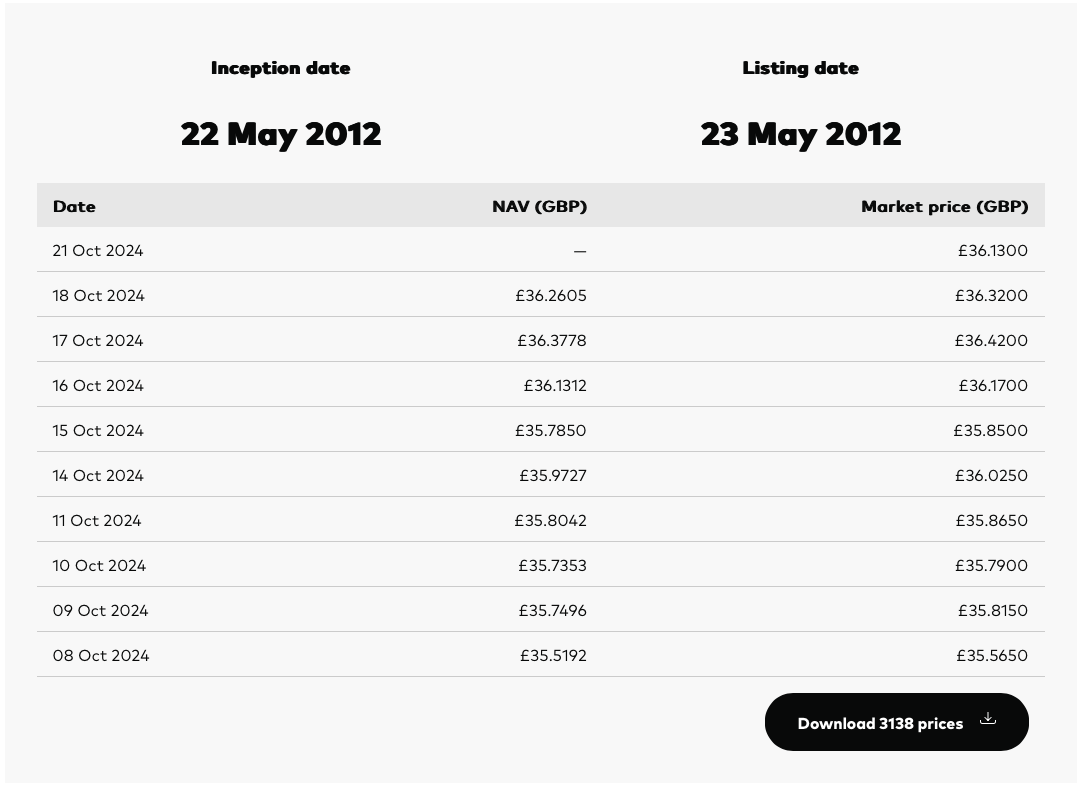
Vanguard update the files nightly with the latest price so there’s no point linking directly to them as the links will become invalid quickly. You can access the latest files here.
The ghost, aka virtual portfolios
Let’s define a ghost or virtual portfolio as one that exists in an alternate world but mirrors exactly the cashflows made in the real world portfolio. The key difference is that in the ghost portfolio, we redirect the cash into a different investment to check our investment performance. Put another way, a virtual portfolio is simply an A/B test for your current investment strategy.
Let’s get into the code
[Note: an earlier version of the code in this article had a bug caused by the use of pandas.merge instead of pandas.concat. I subsequently fixed the bug and also refactored the code using Claude Code which was so interesting I’ve pulled that out into a separate post.]
Given two dataframes A and B, where A holds my personal investment transactions and B contains a reference target - how can I correctly match up transactions made in A with those made in B to enable a direct comparison? A key part of the answer is using the merge_asof built-in function on the pandas DataFrame. It performs an elegant merging of a column from B onto A using key distance. If we order our ‘Date’ column correctly in both Dataframes, we get the complicated merge operation for free!
Here is a partial code listing showing exactly how to do this - it shows how to use the merge_asof function to do some heavy lifting in the analysis. As a rough outline, this code:
- Uses the DataConnectorFactory code written in Part One to load Dataframe A (containing the real-world investments).
- Loads the VUKE data released by Vanguard for daily prices and quarterly distributions.
- Creates Dataframe B as a clone of Dataframe A by using a key Pandas function - merge_asof to emulate the real-world buys and sells.
- Creates a rolling position counter using Pandas cumsum as a precursor to calculating dividends payable per quarter.
- Calculates the dividends.
- Calculates the XIRR for capital only (this is very interesting for the FTSE 100 - see below).
- Calculates the XIRR for capital + distributions.
def run_comparison():
    """
    Run a comparison of actual portfolio against a benchmark index
    """
    # We only need the real buys+sells for the ghost / virtual analysis, not income
    connector = DataConnectorFactory.get_connector("moneywiz")
    df_buys_sells, _ = connector.get_data()
    df_buys_sells["Date"] = pd.to_datetime(df_buys_sells["Date"])

    # Create a comparator using our factory
    comparator = ComparatorFactory.get_comparator("ftse-100")

    # df_virt_cap contains all the buys and sells from the original (source) portfolio
    # re-created for the new virtual portfolio
    df_virt_cap = comparator.virtual_capex_from(df_buys_sells)

    # df_virtual_income contains all of the income generated from the virtual portfolio
    # by calculating units held at each distribution date and multiplying that by the
    # distribution amount
    df_virtual_income = comparator.virtual_income_from(df_virt_cap)

    # Add in the balancing txn if we sold everything today
    num_vuke = df_virt_cap.loc[len(df_virt_cap) - 1, "vuke_position"]
    # Use the latest price to add a final balancing transaction
    # where we liquidate the entire virtual portfolio so that the virtual XIRR is correct
    latest_price = comparator.get_latest_price()
    capital = num_vuke * latest_price
    log.info(f"{num_vuke=}, {latest_price=}, {capital=}")
    sell_all = {"Date": today, "Amount": capital}
    cap_invested = df_virt_cap.Amount.sum()
    # Actually set the final balancing txn
    df_virt_cap.loc[len(df_virt_cap)] = sell_all

    # Let's calc XIRR on capital only (ignoring dividends / distributions)
    xirr_capital = xirr(df_virt_cap[["Date", "Amount"]])
    log.info(f"Ghost portfolio: XIRR on capital only is {xirr_capital*100:.2f}%")
    # Let's see what the return (cap only) is
    capital_rtn_pc = ((capital + cap_invested) / -cap_invested) * 100
    log.info(f"Ghost portfolio: capital return is {capital_rtn_pc:.2f}%")

    # Now let's consider distributions (income) along with capital
    total_income = df_virtual_income["Amount"].sum()
    total_profit = capital + total_income
    total_rtn_pc = ((total_profit + cap_invested) / -cap_invested) * 100
    log.info(f"Ghost portfolio: capital+income return is {total_rtn_pc:.2f}%")

    df_virt_cap_inc = pd.concat(
        [
            df_virt_cap,
            df_virtual_income,
        ],
    )
    df_virt_cap_inc.to_csv("xirr_input.csv")
    df_virt_cap_inc = df_virt_cap_inc[["Date", "Amount"]]
    df_virt_cap_inc = df_virt_cap_inc.sort_values(by="Date", ascending=True)
    assert len(df_virt_cap_inc) == len(df_virt_cap) + len(df_virtual_income)

    # Sanity-check - see if 0-vals are causing xirr() issues
    before = len(df_virt_cap_inc)
    df_virt_cap_inc = df_virt_cap_inc[df_virt_cap_inc.Amount != 0]
    after = len(df_virt_cap_inc)
    if after < before:
        log.info(f"{before - after} 0-val txns removed")
    log.info(f"{df_virt_cap_inc["Amount"].sum()=}")
    log.info(f"{len(df_virt_cap_inc)=}")

    xirr_cap_income = xirr(df_virt_cap_inc)

    log.info(f"Ghost portfolio: XIRR on capital+income is {xirr_cap_income*100:.2f}%")
This code is nice and readable and admits the possibility of plugging in new data providers (S&P 500, NASDAQ, VWRP) in the future. The code that it relies on follows:
class Comparator(ABC):
    """Abstract base class for portfolio comparators"""

    @abstractmethod
    def virtual_capex_from(self, df_buys_sells):
        """Convert buy/sell transactions to virtual portfolio transactions"""
        pass

    @abstractmethod
    def virtual_income_from(self, df_virtual_buys_sells):
        """Calculate income from virtual portfolio transactions"""
        pass

    @abstractmethod
    def get_latest_price(self):
        """Get the latest price for liquidation calculation"""
        pass


class FTSEComparator(Comparator):
    """FTSE 100 comparator implementation using Vanguard FTSE 100 ETF (VUKE)"""

    def __init__(self):
        # Load the VUKE price data using read_excel
        self.df_vuke = pd.read_excel(
            "./data/Historical Prices - Vanguard FTSE 100 UCITS ETF (GBP) Distributing - 07_03_2025.xlsx",
            # More messiness - skip first 8 rows
            skiprows=8,
        )
        # See what we're dealing with
        log.info(f"{self.df_vuke.columns=}")
        # Add in day pricing for VUKE before VUKE started trading
        # Values derived from https://investing.thisismoney.co.uk/historic-prices/UKX?from=2010-08-01&to=2012-08-01
        self.df_vuke = add_out_of_band_txns(self.df_vuke)
        # preprocess_vuke is an analogue of preprocess_vuke_income
        self.df_vuke = preprocess_vuke(self.df_vuke)

        # Store latest price for use in calculations
        self.latest_price = self.df_vuke.loc[0, "vuke_price"]

        # Load the VUKE distribution data
        self.df_vuke_income_raw = pd.read_excel(
            "./data/Distribution History - Vanguard FTSE 100 UCITS ETF (GBP) Distributing - 07_03_2025.xlsx",
            # Messy format from Vanguard - skip first 5 rows
            skiprows=5,
        )
        log.info(f"{self.df_vuke_income_raw.columns=}")
        # Process the income data
        self.df_vuke_income_raw = preprocess_vuke_income(self.df_vuke_income_raw)

    def virtual_capex_from(self, df_buys_sells):
        # Assign VUKE price on actual purchase date to the df, using merge_asof to get the closest match
        # This single line is the beating heart of this code!..
        df_buys_sells = pd.merge_asof(
            df_buys_sells,
            self.df_vuke[["Date", "vuke_price"]],
            on="Date",
            direction="nearest",
        )
        # Make sure our shizzle so far is correct
        assert len(df_buys_sells.loc[df_buys_sells.vuke_price.isna()]) == 0

        # Multiply by -1 here to negate the negative sign of Amount (- means a purchase)
        df_buys_sells["vuke_shares"] = (
            df_buys_sells["Amount"] / -df_buys_sells["vuke_price"]
        )
        # Now use cumsum to get a rolling balance of all VUKE shares over time as we buy and sell
        df_buys_sells["vuke_position"] = df_buys_sells["vuke_shares"].cumsum()
        df_virtual_buys_sells = df_buys_sells[
            ["Date", "Amount", "vuke_position", "vuke_shares", "vuke_price"]
        ]
        return df_virtual_buys_sells

    def virtual_income_from(self, df_virtual_buys_sells):
        # Use merge_asof again to merge real holdings onto the distributions dataframe
        # so we can see how much dividends to "earn" at each Vanguard distribution date
        df_vuke_income = pd.merge_asof(
            self.df_vuke_income_raw,
            df_virtual_buys_sells[["Date", "vuke_position"]],
            on="Date",
            direction="nearest",
        )
        df_vuke_income["Amount"] = (
            df_vuke_income["vuke_position"] * df_vuke_income["amount_per_unit"]
        )
        return df_vuke_income

    def get_latest_price(self):
        return self.latest_price


class ComparatorFactory:
    """Factory for creating portfolio comparators"""

    @staticmethod
    def get_comparator(name):
        """
        Get a comparator by name

        Args:
            name: The name of the comparator to get (e.g., "ftse-100")

        Returns:
            A Comparator instance

        Raises:
            ValueError: If the comparator is not supported
        """
        if name.lower() in ["ftse-100", "ftse100", "ftse 100"]:
            return FTSEComparator()
        else:
            raise ValueError(f"Comparator '{name}' not supported")
Output
Here’s the output when run against a real portfolio and the FTSE 100:
10-03-2025 20:34:17, Ghost portfolio: XIRR on capital only is 3.55%
10-03-2025 20:34:17, Ghost portfolio: capital return is 17.95%
10-03-2025 20:34:17, Ghost portfolio: capital+income return is 36.08%
10-03-2025 20:34:17, 35 0-val txns removed
10-03-2025 20:34:17, Ghost portfolio: XIRR on capital+income is 7.31%
So for the FTSE 100 starting in 2012, the XIRR on capital alone is 3.55%. We can see that dividend distributions form a significant part of the total return generated and the overall XIRR for this ghost portfolio is 7.31% when both capital returns and dividends are combined.
Findings / Analysis
[Note to reader: this section has been re-written from v1 to reflect the bug identified and fixed..]
So, down to brass tacks - how does this theoretical return compare with the actual return generated by the real portfolio? As of today (10th March 2025), the real portfolio XIRR is 7.35% (!!), so the FTSE 100 ghost portfolio just barely underperforms my actively-managed portfolio by 0.04% or 0.5% relative.
That’s a tiny difference overall. Investing in the FTSE 100 index should be statistically safer with the risk spread out over 100 large-cap constituents. I’ve re-run the analysis for different time periods and there are date ranges when I outperform the index and vice versa, but inevitably, inexorably the index will always win out in the end as the time horizon extends.
As an example, the real truth is that I cannot in all good conscience distinguish clearly between my two best performers (both up over 600%, both defence / aerospace) and my two biggest losers (both down over 90% - one exposed to bad UK government decisions, one to the retail property market during COVID). I bought all 4 stocks thinking they were winners and was wrong 50% of the time.
Lastly, I have to watch and manage this portfolio quite a bit and respond regularly to corporate actions (dilutive events, cash returned as capital (why?) etc.) - buying an ETF that tracks the market is just “set and forget” with pretty much exactly the same return. ETFs in the UK are also not subject to the initial 0.5% stamp duty tax.
Conclusion
I use the code from Part One regularly. That code, and the ghost comparison code in this post, really helped me to understand my investing performance for what I consider to be a lower-risk side of my portfolios (private investing in startups is much more risky but also much more lucrative).
Lastly, a comparison to an S&P 500 tracker or a world-wide tracker like VWRP (which is 70% US anyway) will show a far greater disparity in investment performance but truthfully I do look at the FTSE 100 a lot. I’ve considered the US markets to be frothy for a long time now and Shiller / CAPE ratios indicate that a reversion to mean is on the cards but you cannot time the market..
Summary
In summary, in part one we calculated XIRR at both the individual ticker level and portfolio level. In Part Two (this article), we extended the XIRR analysis to perform a comparative analysis vs a major benchmark index - the FTSE 100 in the UK. Conducting this analysis enforces an investing discipline that otherwise wouldn’t exist. It’s amazing to think that investment platforms do not provide XIRR numbers routinely - they are a key part of understanding (and thus improving) your personalised investment performance.